The Governance Risk Framework: Part 2¶

“The first principle is that you must not fool yourself — and you are the easiest person to fool.

So you have to be very careful about that. After you’ve not fooled yourself, it’s easy not to fool other scientists.

You just have to be honest in a conventional way after that.”

Richard P. Feynman — On scientific integrity.

14 June 1974, Caltech, California, USA

Introduction¶

In the first part of this three-part series, we covered the stablecoin universe, defined decentralized risk management and outlined the governance structure around the risk function. In this article, the second part of the series, we will take a more in-depth look at the risks underlying the system — Describing how parameters in the MakerDAO system encapsulate those risks. Then finally outline the models that are most appropriate for measuring and managing those risks. To start, we go straight to the heart of the system, the CDP, and discover the dangers we face in supplying Dai.

The Inherent Risks Of Supplying Dai Using CDPs¶

Traditionally, loans are made with sufficient collateral in place to minimize the exposure at the time of default. The question is, what makes that collateral sufficient? Collateral is adequate when there is enough of it to cover all of a loan if ever that loan is placed into default. Which seems simple enough, if I pledge $100 worth of gold, would you lend me $100? Immediately you would say ‘no’ — because the price of gold fluctuates and at any point in time you could have less gold than the amount you lent out. If a default occurred at such a precarious time, you would not be able to recover the full loan. The obvious solution is to ask the borrower to pledge more gold to cover the volatility of gold’s value. So the first risk factor we need to consider would be the volatility in the value of the collateral.

Gold is purposefully used as an example, as it holds a lot of assumptions that most of us take for granted. The first assumption is that gold will remain, well, ‘gold’. What is meant by that? It is possible to replace gold in its industrial use and as a store of value — if that happened the value of gold would become quite volatile and possibly drop — it’s just not probable that it would occur any time soon, but we need to be cognizant of gold’s fundamental qualities. The second assumption about gold is that given the primary attributes of gold, there is a liquid marketplace where we could turn gold into fiat currency. Without sufficient liquidity, the price of gold will not reflect its real value. Think of it this way, the price is an advertisement, but the value is what you will get for it. That creates two more risk factors for us to consider, the first is the risk of change in the qualitative characteristics of the token, and the second is the risk of change in the liquidity of the token.

There is another feature of gold we take for granted that is indirectly related to liquidity. The value of all the gold ever mined is roughly $7.5 trillion. So, from any one person’s perspective, it’s highly improbable to own a majority stake in gold or even a significant amount of gold relative to the total supply.

Unlike gold, the MakerDAO system could find itself with a concentrated position in a particular token if the majority of its owners used it as collateral. For example, if a crypto token with an available supply of $100m in the market had a substantial portion of the owners use this token as collateral, MakerDAO would have real exposure to this token. If, say, $40m of this token is collateral, and the collateral value started dropping rapidly, it should be clear that trying to get rid of 40% of the available supply (even in a liquid market) would directly impact the price and cause a downward price spiral. Thus the fourth risk factor to include is the risk of a concentrated exposure.

We now understand the risk of taking on too much exposure to one collateral type. Another is taking exposure to only ONE collateral type, which is where diversification is needed. We know that many volatile assets held in a portfolio create a diversification benefit. Simply put, the lower the correlation between tokens the more significant the diversification benefit. Multi-collateral Dai will use different tokens, so the fifth risk factor to include is correlation risk, or in other words the risk of change in the diversification benefit.

The final risk and something that is especially relevant to the crypto space, is price feeds. The US market has a fragmented securities exchange structure. There are multiple venues where one could complete a transaction in stock, resulting in the need for a ‘Securities Information Processor’ or SIP in the US. The purpose of this entity is to aggregate the best bids and offers from all the exchanges and disseminate the best bid and offers to the appropriately licensed data vendors. In turn, regulating information distributed to the public. The crypto space is itself fragmented, but at the moment there is no SIP in place to authenticate and monitor the data sent to the public — requiring the need to self-regulate prices. Till then, the quality of the feed dictates the value of the collateral underlying the loan. If we can’t depend on the feed, we can’t depend on the prices, and we thus have no confidence in the value of the collateral.

To summarize, the risks inherent in supplying Dai are as follows:

• Volatility risk: the higher the volatility of the collateral value, the less likely we are to recover the full loan in the event of default.
• Qualitative risk: the less stable the fundamentals of the organization, the less confident holders will be, and the more volatile the price will become.
• Liquidity risk: the less liquidity available in the market, the more likely the price impact will work against realizable value.
• Exposure risk: the higher the aggregate relative exposure to total supply, the more risk in trying to realize its value.
• Correlation risk: the higher the correlation, the less the diversification benefit.
• Price feed risk: low quality feeds create low confidence in value.

It probably has become apparent that the risks stated above are interrelated. If you start with one risk you could easily deduce the effect it could have on the others.

We need to understand how to identify, measure, and manage the above-mentioned risks so that Maker token holders understand the exposures they face and the information available to make decisions. The sections that follow will outline each of these risks, the suggested risk management model and to what extent the risk parameters encapsulate these risks. Furthermore, we will outline the duties required from both the internal risk team and Maker token holders.

We will cover the risks in the order that is in line with how tokens are on-boarded as collateral. First, we start with the qualitative risk, then the exposure risk, liquidity and volatility risks together, correlation risk, and finally, the price feed risk.

Exploring The Inherent Risks And How To Manage Them¶

Qualitative Risk¶

QR: Outline¶

To evaluate if the token will continue to operate with the same character as it has before (think of gold), we need to understand and assess the organization behind it. Doing a full evaluation for an investment is to combine due diligence of the organization with a financial analysis. The purpose of the financial analysis is to deduce a fair value for the token — the goal of the due diligence is to understand the potential volatility around that fair price due to operational and business risks. For MakerDAO, we are more interested in the inherent instability due to operational and business risk. We will leave the price opinion and price formation for the market to decide. To ascertain the business risks of the organization we need to abstract all the features of the organization — then distill them until we can understand a clear picture of the risks surrounding the token.

QR: Risk Management Function¶

The necessary function here is to facilitate and contribute to the compilation of information to assess the qualitative features of the organization behind the token used as collateral. The process to compile data through due diligence has three parts and is conducted sequentially to use resources as efficiently as possible.

The three parts are:

• The Initial Collateral Onboarding Process: this covers the trade support structure, distribution of token holdings and available data series.
• The Operational Assessment Process: this covers the functionality behind the token, from the organization itself, through to the governance mechanisms and rights of the token owner.
• The Technological Assessment Process: this covers the robustness and security of the underlying technology.

The information compiled from the due diligence will be used to rate the features of the potential collateral token. The features of the organization to assign a rating to are:

• Team — Core team and advisors.
• Community — Sentiment analysis.
• Technology — Security and completeness review.
• Market and Competitiveness — SWOT analysis.
• Business Models — Structural and legal analysis.

Assigning a rating to each feature will result in an overall rating. A score below a prerequisite value will place the token to the back of the queue, and a passing score is an adjustment factor to the risk parameters of the system. We will elaborate on the features and rating system in a forthcoming document. For now, the point is to communicate the process.

Maker token holder (MTH) and Maker internal risk team (MRT) duties¶

MRT will create a qualitative risk template and assign ratings on this template. The model and information will be made available for MTH and other teams to use for themselves. Ultimately the risk function, made up of many groups, will collectively produce a weighted group rating for the token.

MTH will use the available information, along with the collective rating to decide whether to include the token into the collateral portfolio. As mentioned a rejected token will go to the back of the queue; otherwise, collateral will be included in the portfolio or assigned to be ‘reviewed.’ On ‘review’ means no decision made because of an impasse, or not enough information was available to make the decision.

Exposure Risk — Debt Ceiling¶

ER: Outline¶

How much exposure of one collateral type are we willing to take? When is too much? What does ‘too much’ mean?

This concept of ‘too much’ represents the level of exposure relative to the available supply.If we breach that level, then we have an untenable concentration in exposure to one collateral type. It is unsustainable for if we attempted to liquidate it, it would impact the market so much (even a liquid market) that it would likely drop the value of the token to the extent that would not allow us to realize the full amount of the loans collateralized by that token.

This level of collateral exposure is called the Maximum Exposure Level, and given the Liquidation Ratio (explained in next section), we can calculate the Dai exposure level as the Debt Ceiling, which is the maximum amount of Dai that should be lent out given this collateral type. This level is not absolute, and it is related to the available supply.

To take it one step further, we need to consider the relationship between liquidity and free float. Free float is the readily traded portion of the available supply of tokens — the amount not held over the long term by founders and large institutions. Therefore any real liquidity presented in the market is a result of the free float.

There is a top-down and bottom-up approach to calculating the Debt Ceiling. The top-down starts with the free float and asks, ‘What is the maximum proportion we are willing to hold?’ The bottom-up starts with price impact and asks, ‘What is the maximum impact you think the market could sustain on a daily basis over a given period?’

Generally, the top down and bottom up approach don’t meet ‘in the middle,’ in fact, the top down should be seen as a constraint on the bottom up. If the bottom-up approach suggests the market is liquid enough to absorb a large number of tokens, but that amount is substantially more than the relative exposure to supply you are willing to hold — then stick with the top-down approach.

ER: Risk Management Function¶

The calculation of the debt ceiling for a single token considers three practical issues. The first is the calculation of the highest debt ceiling given the assumption that the token has the liquidity for it. A calculated value based on the top-down approach that we have just discussed and we call it the Theoretical Debt Ceiling. The second issue is to consider what the current trading environment and portfolio permit the maximum level to be — this is related to the bottom-up approach — and known as the Practical Debt Ceiling. It considers the current trading environment as well as the current collateral portfolio risk profile. The last issue involves considering the rate at which the current Debt Ceiling increases. If the Debt Ceiling rises too quickly, it may be due to increased speculative activity or even an aggressive attack vector. In short, the rapid rate of increase could be indicative of an attack vector or an abnormal rise in volatility. Both of which would present problems to the system. Therefore the rate at which the debt ceiling may increase will be constrained by the Defensive Debt Ceiling, as an example, we could perform the calculation as follows:

Where the ‘constrained rate’ will capture the maximum rate of increase over a given period.

In summary, the Theoretical Debt Ceiling is the maximum token based supply of Dai allowed for a particular token. The Practical Debt Ceiling is the limit that the market for that token can handle at that time, and the Defensive Debt Ceiling looks after the system as the debt level grows.

We will present the model used by the internal risk team to calculate these ceilings in a forthcoming paper.

ER: Maker token holder (MTH) and Maker internal risk team (MRT) duties¶

MRT will create the debt ceiling model as a template, and make it available to other teams and MTH. Further, MRT will educate MTH and any other interested participants on the workings of the model through various mediums and communication channels. Collateral that passes the qualitative assessment will have its debt ceilings calculated by the decentralized risk function, which initially will be MRT, but ultimately resulting in a weighted average of contributions by all the teams in the risk function.

The debt ceiling model will be a part of the risk construct presented by a risk team. Recall the risk construct is a collection of models used to calculate one or more of the risk parameters for the system. Once MTH vote in a risk team they adopt the risk construct and values derived from those models in the construct. MTH will understand the constructs and the underlying models through various communications with the different risk teams. Furthermore, MTH will also be involved in the debate amongst the various risk teams.

Liquidity and Volatility Risk — Liquidation Ratio¶

LVR: Outline¶

The Debt Ceiling controls the risk of creating an illiquid market due to holding too much of one token or creating the effect of an illiquid market by liquidating too much inventory. Liquidity risk evaluates the current liquidity of the market, where Volatility risk assesses the price risk (market risk) of the token given the level of liquidity in the market.

The amount of collateral required for a particular token is dependent on both volatility and liquidity risks. We address the volatility aspect by revisiting the gold example. How much gold would be needed to collateralize a $100 loan? Well, if the volatility of the price of gold is 10% per day, you would probably want something in the region of $125. Given you are conservative, you would probably want twice the volatility of the daily price incorporated into the collateral value. Which is conservative as the chance of the price falling by 20% in one day is very remote — possible — but remote. Back to the example, the collateral we would need would be $100/0.8 = $125, or, put another way, starting at $125: if the collateral value drops by 20% that would equal a $25 loss in value but we would still have \$100 in value which is enough to cover the outstanding loan, given nothing is paid back.

Now we include the Liquidity Risk Factor. We have assumed that $125 of gold would be sufficient to cover the $100 loan. What about a $1m loan? Well we know the amount of collateral we would need is $1.25m, but getting rid of $1.25m in gold is a more complicated problem than getting rid of $125 of gold. We have to consider the liquidity of the market yet again. So what is required is an adjustment of the collateral value to compensate for liquidity risk. To carry on the example, assume the liquidity adjustment is 1.15 or an increase of 15% in value. Then the final collateral value required would be \$1.435m.

Given the volatility risk, and a uniform application of the liquidity risk adjustment, we have determined that to borrow $100 one would need to pledge $143.50 in collateral.

The one outstanding issue is the duration of the loan. If the loan is longer than a day, then clearly more collateral would need to be posted — or at least we would require an adjustment to the collateral on a daily basis. Considering the loans in the MakerDAO system are open-ended, does that mean that we need a massive amount of collateral? The short answer is no, unlike the traditional setting, a loan is liquidated immediately if a default occurs. The applicable period to consider is then the length of time to liquidate the position. So we will include a predetermined maximum amount of time to liquidate the position and adjust the collateral calculation for it.

To summarize, from volatility risk we can calculate the initial amount of required capital, from liquidity risk we can make a liquidity adjustment to the calculation. Given the length of time to liquidate that collateral, the final change would be the time — or expected liquidation period.

LVR: Risk Management Function¶

How does this all relate to the liquidation ratio? The liquidation ratio is the required amount of collateral as a proportion of the loan. So in our example, if we consider that from volatility the necessary amount of gold as collateral was $125. Then after adjusting for liquidity, it was $143.50, then adjusting for the expected liquidation period it turned out to be $175. The liquidation ratio would then be $175/\$100 = 175%. So the liquidation ratio can be generally approximated by:

Where the VaR term is the value at risk at a given confidence level, an idea and calculation we will explore further in a more detailed paper focussed on the liquidation ratio.

Participants in the system liquidate the collateral if the collateral to debt ratio falls to or below this level. A level that ensures, given certain confidence, the collateral when liquidated should be sufficient to recover the loan. With any excess collateral returned to the borrower. If the collateral is insufficient, MKR token holders will be diluted to make up for any outstanding part of the loan that has not recovered. As mentioned, the details of the model will be discussed in a forthcoming paper.

LVR: Maker token holder (MTH) and Maker internal risk team (MRT) duties¶

In the same fashion as the debt ceiling, MRT will create the liquidation ratio model as a template, and make it available to other teams and MTH. Further, MRT will educate MTH and any other interested participants on the workings of the model through various mediums and communication channels. Collateral that passes the qualitative assessment will have its liquidation ratios calculated by the decentralized risk function, which initially will be MRT, but ultimately resulting in a weighted average of contributions by all the teams in the risk function.

The liquidation ratio models will be a part of the risk construct. Again, when MTH votes in a risk team, they adopt the risk construct and values derived from those models in the construct. MTH will understand the constructs and the underlying models through various communications with the different risk teams. Furthermore, MTH will also be involved in the debate amongst the risk teams.

Correlation Risk¶

CR: Outline¶

If you create a portfolio of two financial assets, the risk of that portfolio will almost always be less than the sum of the individual risks of the underlying assets. The reason, the correlation of returns between two different assets are generally never perfect. The result is a diversification benefit for the portfolio. We can express that diversification benefit as follows:

The expression shows the benefit as the portfolio volatility subtracted from the sum of the individually weighted volatilities. Where the portfolio volatility includes diversification, and the sum of weighted volatilities assumes no diversification. So by subtracting we get the diversification benefit denominated in units of volatility saved.

If the correlation between the two assets stayed the same forever, we would then have a constant diversification benefit. But correlation changes, resulting in the diversification benefit changing. Creating a risk to the portfolio, specifically, the risk of correlation increasing.

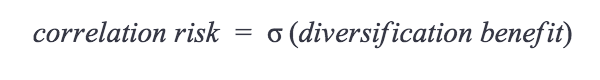
The higher the correlation, the less the diversification benefit. So correlation risk is defined as the volatility of the diversification benefit.

The way to manage correlation risk is by adding more collateral types to the portfolio that have either nothing in common with it or act in opposition to it. With the goal that once a critical mass of unrelated collateral types are in the portfolio, the diversification benefit will stabilize.

The MakerDAO system will use multiple tokens as collateral. Making the objective clear, to include as many uncorrelated tokens as possible. Unfortunately, this is something easier said than done as we shall explore next.

CR: Risk Management Function¶

Understanding how to manage correlation risk requires a working definition of book-building and risk capital. Book-building is the way you include assets in the portfolio. There are many techniques to do this, but mainly it requires keeping your portfolio within a risk/return framework until it is complete. Risk capital is the amount of actual capital that an organization wishes to risk to remain solvent to attain an expected return. Risk capital also known as economic capital will be covered more extensively in the final section of this article.

We can now combine the concepts. If you book-build a collateral portfolio within a determined risk/return framework, you will consume your risk capital efficiently. Each collateral type will have a distinct stability fee, representing the return component to the organization. Given the stability fee, if the risk profile of the collateral type contributes to the diversification of the portfolio, without materially affecting the overall return, it will be included. The extent to which it’s involved depends on the amount of risk capital it consumes.

Assume a given level of risk capital. If we start with a small group of highly correlated tokens — it could quickly use up the risk capital with little diversification benefit. Ideally what you want, is to build the collateral portfolio uniformly, of uncorrelated tokens to get the best diversification benefit. Ideal, but far from being a business reality. Unlike the traditional equity space, we are not spoiled for choice and have to settle for what is available. And what is available, at least in the beginning will have a higher than average level of correlation.

CR: Maker token holder (MTH) and Maker internal risk team (MRT) duties¶

MRT will provide a portfolio tool and suggest potential collateral types that are a best fit based on that tool. Further, MRT will educate MTH and any other interested participants on the methods used through various mediums and communication channels.

The portfolio tool will contribute towards the qualitative assessment and be a part of the risk construct. Again, when MTH votes in a risk team, they adopt the risk construct and values derived from those models in the construct. MTH will understand the constructs and the underlying models through various communications with the different risk teams. Furthermore, MTH will also be involved in the debate amongst the risk teams.

Price Feed Risk¶

PFR: Outline¶

There is a difference between price and value. Price is an advertisement and very seldom the amount that you will realize. This characteristic is particularly crucial in crypto markets where the fragmented exchange system has given rise to many sources of price information.

Consequently, there are many techniques made available to ascertain a more representative sense of value from all these price sources. Still, it remains to evaluate such methods for the inherent and implicit risks they bring.

How do you assess the quality of information a source brings? How long will that source be around?

The quality of the information from a price source does not end with its accuracy against transactional evidence seen in the market. It concludes by acknowledging that some of the transactional evidence itself may be misleading due to wash trading. Given that the transactional evidence is authentic and the price source relays that information appropriately — is it the primary job or function of the entity to provide the source? If not, that source could readily disappear. Imagine where the financial world would be if Bloomberg just disappeared tomorrow.

Therefore the risk is in the quality of the information at the source level, the exchange level and concerning longevity. Strictly speaking, this is more of a technical problem, but it is such a significant risk that it spills over into all parts of the business including financial and economic risk management.

PFR: Risk Management Function¶

Currently, the management of this risk is done by vetting multiple sources and taking the median of the price with a delay mechanism. Taking a cross-section of the multiple sources and applying the median ensures unrealistic size differentials does not bias the result as it would with averaging, the following unbiased and unbiased sets show an example of the fact:

The delay mechanism allows for the comparison of the delayed price to the current price. Which allows enough time to identify an attack vector in price and do something about it, before using the delayed price.

PFR: Maker token holder (MTH) and Maker internal risk team (MRT) duties¶

MRT will present the first technique and process to manage the feed risk. Then continually research and update the method when necessary. Further, the team will educate MTH through various mediums and communication channels.

MTH may vote intermittently to adopt new oracles and transformations to manage feed risk.

Economic Capital and the Stability Fee¶

EC: Outline¶

What is economic capital? A term straight from the literature of financial risk management, it is the amount of capital that an entity risks to remain solvent to attain an expected return. Economic capital is also known as risk capital. There is a decision involved here, however, and it relates to the level of risk aversion of an organization. The more risk averse the organization, the less economic capital deployed.

The MakerDAO system is designed to cover excess outstanding loan amounts not covered by the liquidation of collateral. Keep in mind that the collateral initially pledged renders an extremely low probability of it NOT being sufficient to cover the loan in the event of a default, this is where risk or economic capital comes in. We can now phrase the question clearly, how much capital must be set aside for the operation to remain solvent if the collateral is not sufficient?

The type of events we are talking about here are tail events or stress events. These are the events that are considered highly unlikely, and to a certain extent could represent events never seen before. The way you calculate the economic capital is by calculating the expected value of loss given a tail event. There are no guarantees, what we are doing is covering for risk using collateral and then covering for the risk of risk itself being risky (yes — I just wrote that) with economic capital.

EC: Risk Management Function¶

Economic capital represents the amount of risk an organization is prepared to take, so what does it expect to get in return? Each loan in MakerDAO attracts a stability fee. A fee that is charged to compensate MakerDAO for operating and maintaining the stability of the system. The stability fee is similar to an interest rate, and an interest rate is made up of a couple of components. In short, an interest rate must compensate for purchasing power, so it must first pay for inflation. The second component is the operating cost and policy instrument of the organization. The third is a premium that is paid to compensate Maker token holders for providing the above-mentioned insurance. Traditionally this would be a credit risk premium attached to the borrower’s credit quality, but in this system, the credit risk is shifted entirely to the collateral. Further, the traditional method would have a liquidity preference fee, which creates a higher compensation for more extended loans. Again, in the MakerDAO system, this does not apply, as the loans are facilities that are open-ended.

To summarize, the credit stability fee simplistically can be seen as the sum of the inflation rate, operational cost premium, and credit insurance premium.

The credit insurance premium component is more applicable to our context at the moment. For the ease of exposition, let’s assume inflation and the cost to operate the organization is zero. We then consider the stability fee as just a premium that pays the system to provide the insurance if the collateral is not sufficient. A way of understanding the stability fee is thinking of it as the probability that MakerDAO will use all of its risk capital (given a few assumptions we won’t address here). An easy way to think of this is in terms of expected loss. Assuming all the risk capital used, we represent expected loss as:

So if we use a nominal value for risk capital — say $100, then the expected loss is $2.50 if the probability of the event is 2.5%. Clearly showing that \$2.50 or instead 2.5% is the appropriate compensation per year for taking on such risk.

Now the way the economic capital and stability fee relate to each other is through this interpretation of probability. Remember if we think of the stability fee as a probability that we would use all the risk capital then we would want the expected value of our business to be positive that is:

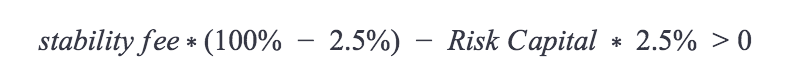
The above inequality represents two events. The first term, is no event of default, over a one year period, where we earn a stability fee. The second term is the event of default within a one year period and uses all the risk capital. Note the events are mutually exclusive in this exercise. Either a default occurs, and we use the risk capital, or it does not.

Given that stability fee (which is equivalent to the probability of default) is 2.5% per year the risk capital inequality resolves to:

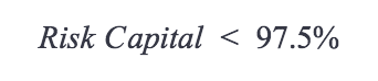
Risk Capital should be 97.5%/2.5% = 39x higher than the stability fee. A quick calculation (by taking the reciprocal) shows a return on risk-adjusted capital of 2.56% (2.5%/97.5%) — not a very attractive return. Still, there is a simple intuition missing here. Let’s rephrase the full inequality again with one addition:

Then our risk capital term would be defined as:

The above shows that risk capital represents the part of the loan that collateral does not cover. The resolved inequality (Risk Capital < 97.5%) then states that risk capital should be less than 97.5% of the outstanding loan! Well, this should be the case as we hope that the collateral will cover the lion’s share of the risk. We would expect that risk capital would represent a relatively small portion of the outstanding loan. Conservatively the proportion would not exceed 8–10% of the outstanding loan. Far less than the Risk Capital < 97.5% requirement. In fact, if we take the upper value of 10% and recreate the return reciprocal, the return on risk-adjusted capital would be (2.5%/10%) 25% — a more attractive yield.

The economic capital calculation is a top-down tool used to calculate the stability fee for each collateral type. Further, it can be used to assess the minimum stability fee for the portfolio as a whole. It should be clear how it relates to the diversification benefit previously introduced with the correlation risk factor. In fact, it may have become more evident how the Debt Ceiling, Liquidation Ratio, Correlation Factor, and Economic Capital are fundamental inputs into continually building, managing and diagnosing the collateral portfolio underlying the MakerDAO system.

EC: Maker token holder (MTH) and Maker internal risk team (MRT) duties¶

MRT will create the methodology and templates to calculate the economic capital and stability fee and make it available to other teams and MTH. Further, MRT will educate MTH and any other interested participants on the workings of the model through various mediums and communication channels. Collateral that passes the qualitative assessment will have its stability fee calculated by the decentralized risk function, which initially will be MRT, but ultimately resulting in a weighted average of contributions by all the teams in the risk function.

The stability fee calculation will be a part of the risk construct. Again, when MTH votes in a risk team, they adopt the risk construct and values derived from those models in the construct. MTH will understand the constructs and the underlying models through various communications with the different risk teams. Furthermore, MTH will also be involved in the debate amongst the risk teams.

Conclusion¶

Every organization faces a set of risks, or rather, layers of risk. In this second part of the series on the Governance Risk Framework, we focused on the risks inherent in the supply of Dai using CDPs. Which is the layer of risk directly attributable to the engine of the MakerDAO system. The risks identified were then encapsulated either into the risk parameters of the system or placed in the correct context of the system. The responsibility of the internal risk team, as well as Maker token holders, were outlined. With an emphasis on future papers to be delivered that will detail the models used for the primary risk parameters in the system.

The third and final part of this series will look at the decisions facing Maker token holders. It will detail the types of decisions, ranging from the initial decisions about the internal risk team, through to the more regular choices concerning collateral types. Elaborating on the different votes available and the expected timing of those votes. It will then wrap up with how the entire risk function will operate under the careful deployment and management of the scientific risk governance process by the Maker token holder community.